

Time Series#
A time series is a sequence of data points recorded over time — for example, a temperature sensor logging every 15 minutes or an electricity meter sending hourly readings.
In practice, time series data does not always come at regular intervals. IoT sensors, LoRaWAN devices, and event-based systems often transmit data at irregular timestamps — depending on signal quality, battery level, or only when a value changes. This makes it essential to align and regularize timestamps before analysis.
pandas provides powerful tools for this: resampling to a fixed frequency, interpolating gaps, computing rolling statistics, and aligning multiple series to a common time axis.
# Load data set

import pandas as pd

df = pd.read_csv("https://raw.githubusercontent.com/retomarek/edap/main/edap/sampleData/flatTempHum.csv",
                 sep = ";")
df['time'] = pd.to_datetime(df['time'], format='%Y-%m-%d %H:%M:%S')

df.head()
| time | FlatA_Hum | FlatA_Temp | FlatB_Hum | FlatB_Temp | FlatC_Hum | FlatC_Temp | FlatD_Hum | FlatD_Temp | |
|---|---|---|---|---|---|---|---|---|---|
| 0 | 2018-10-03 00:00:00 | 53.0 | 24.43 | 38.8 | 22.40 | 44.0 | 24.5 | 49.0 | 24.43 |
| 1 | 2018-10-03 01:00:00 | 53.0 | 24.40 | 38.8 | 22.40 | 44.0 | 24.5 | 49.0 | 24.40 |
| 2 | 2018-10-03 02:00:00 | 53.0 | 24.40 | 39.3 | 22.40 | 44.7 | 24.5 | 48.3 | 24.38 |
| 3 | 2018-10-03 03:00:00 | 53.0 | 24.40 | 40.3 | 22.40 | 45.0 | 24.5 | 48.0 | 24.33 |
| 4 | 2018-10-03 04:00:00 | 53.3 | 24.40 | 41.0 | 22.37 | 45.2 | 24.5 | 47.7 | 24.30 |
Irregular to Regular Time Series#
Real-world sensor data often arrives at irregular intervals. Before you can compare, resample, or plot multiple sensors together, the timestamps need to be aligned to a regular grid (e.g. every 15 minutes).
import pandas as pd
import numpy as np

# Simulate irregular IoT sensor data (LoRaWAN-style)
np.random.seed(42)
irregular_times = pd.to_datetime([
    "2024-01-15 08:02:13", "2024-01-15 08:17:45", "2024-01-15 08:28:02",
    "2024-01-15 08:46:33", "2024-01-15 09:01:11", "2024-01-15 09:14:58",
    "2024-01-15 09:33:27", "2024-01-15 09:44:05", "2024-01-15 10:02:41",
    "2024-01-15 10:19:16", "2024-01-15 10:31:52", "2024-01-15 10:48:09",
])
df_irregular = pd.DataFrame({
    "temperature": [21.3, 21.5, 21.4, 21.8, 22.0, 22.1, 22.3, 22.2, 22.5, 22.4, 22.6, 22.5]
}, index=irregular_times)

print("Irregular timestamps:")
df_irregular
Irregular timestamps:
| temperature | |
|---|---|
| 2024-01-15 08:02:13 | 21.3 |
| 2024-01-15 08:17:45 | 21.5 |
| 2024-01-15 08:28:02 | 21.4 |
| 2024-01-15 08:46:33 | 21.8 |
| 2024-01-15 09:01:11 | 22.0 |
| 2024-01-15 09:14:58 | 22.1 |
| 2024-01-15 09:33:27 | 22.3 |
| 2024-01-15 09:44:05 | 22.2 |
| 2024-01-15 10:02:41 | 22.5 |
| 2024-01-15 10:19:16 | 22.4 |
| 2024-01-15 10:31:52 | 22.6 |
| 2024-01-15 10:48:09 | 22.5 |
# Step 1: Resample to a regular 15-minute grid using the nearest value
df_regular = df_irregular.resample("15min").nearest()

print("Regular 15-min timestamps:")
df_regular
Regular 15-min timestamps:
| temperature | |
|---|---|
| 2024-01-15 08:00:00 | 21.3 |
| 2024-01-15 08:15:00 | 21.5 |
| 2024-01-15 08:30:00 | 21.4 |
| 2024-01-15 08:45:00 | 21.8 |
| 2024-01-15 09:00:00 | 22.0 |
| 2024-01-15 09:15:00 | 22.1 |
| 2024-01-15 09:30:00 | 22.3 |
| 2024-01-15 09:45:00 | 22.2 |
| 2024-01-15 10:00:00 | 22.5 |
| 2024-01-15 10:15:00 | 22.4 |
| 2024-01-15 10:30:00 | 22.6 |
| 2024-01-15 10:45:00 | 22.5 |
Alignment methods
There are several ways to align irregular data to a regular grid:
Method |
Code |
Best for |
|---|---|---|
Nearest |
|
Sensor values that change slowly (temperature, humidity) |
Mean |
|
Multiple readings per interval — averages them |
Interpolate |
|
Smooth signals, fills gaps with linear interpolation |
Forward fill |
|
State data (on/off) — carries last known value forward |
Why is this important? Many analysis methods (resampling, rolling mean, merging multiple sensors) require a regular time index. If two sensors report at different irregular times, you cannot directly compare or correlate them without aligning first.
Datetime Index#
Setting the datetime column as the DataFrame index unlocks powerful time-based features in pandas: slicing by date range (df.loc["2024-01"]), resampling (.resample()), and automatic alignment when combining multiple DataFrames. Without a datetime index, these operations require extra code and are slower.
# set index and remove column
df = df.set_index("time", drop=True)

# remove duplicates
df = df[~df.index.duplicated(keep='first')]

df.head()
| FlatA_Hum | FlatA_Temp | FlatB_Hum | FlatB_Temp | FlatC_Hum | FlatC_Temp | FlatD_Hum | FlatD_Temp | |
|---|---|---|---|---|---|---|---|---|
| time | ||||||||
| 2018-10-03 00:00:00 | 53.0 | 24.43 | 38.8 | 22.40 | 44.0 | 24.5 | 49.0 | 24.43 |
| 2018-10-03 01:00:00 | 53.0 | 24.40 | 38.8 | 22.40 | 44.0 | 24.5 | 49.0 | 24.40 |
| 2018-10-03 02:00:00 | 53.0 | 24.40 | 39.3 | 22.40 | 44.7 | 24.5 | 48.3 | 24.38 |
| 2018-10-03 03:00:00 | 53.0 | 24.40 | 40.3 | 22.40 | 45.0 | 24.5 | 48.0 | 24.33 |
| 2018-10-03 04:00:00 | 53.3 | 24.40 | 41.0 | 22.37 | 45.2 | 24.5 | 47.7 | 24.30 |
Note
The index column with 0, 1, 2 etc. has gone and now datetime is the index!
Upsampling#
Increase the frequency of the samples, such as from hours to 15min
df15min = df.resample("15min").interpolate(method="linear")
df15min.head()
| FlatA_Hum | FlatA_Temp | FlatB_Hum | FlatB_Temp | FlatC_Hum | FlatC_Temp | FlatD_Hum | FlatD_Temp | |
|---|---|---|---|---|---|---|---|---|
| time | ||||||||
| 2018-10-03 00:00:00 | 53.0 | 24.4300 | 38.8 | 22.4 | 44.0 | 24.5 | 49.0 | 24.4300 |
| 2018-10-03 00:15:00 | 53.0 | 24.4225 | 38.8 | 22.4 | 44.0 | 24.5 | 49.0 | 24.4225 |
| 2018-10-03 00:30:00 | 53.0 | 24.4150 | 38.8 | 22.4 | 44.0 | 24.5 | 49.0 | 24.4150 |
| 2018-10-03 00:45:00 | 53.0 | 24.4075 | 38.8 | 22.4 | 44.0 | 24.5 | 49.0 | 24.4075 |
| 2018-10-03 01:00:00 | 53.0 | 24.4000 | 38.8 | 22.4 | 44.0 | 24.5 | 49.0 | 24.4000 |
Upsample methods
When upsampling (e.g. hourly to 15-min), you need to fill the new empty rows. Available methods:
Method |
Code |
Description |
|---|---|---|
Linear interpolation |
|
Straight line between known points — good default |
Spline interpolation |
|
Smooth curve — more natural for sensor data |
Forward fill |
|
Carries the last known value forward |
Backward fill |
|
Uses the next known value |
Nearest |
|
Uses the closest value in time |
Frequency aliases
Alias |
Meaning |
Example |
|---|---|---|
|
seconds |
|
|
minutes |
|
|
hours |
|
|
calendar days |
|
|
weeks (ending on Sunday) |
|
|
month start / month end |
|
|
quarter start / year start |
|
Older code uses "T", "H", "M" or "A": these aliases were renamed in pandas 2.2 and are rejected by pandas 3.
Downsampling#
Decrease the frequency of the samples, such as from hours to days
dfDaily = df.resample("D").mean()
dfDaily.head()
| FlatA_Hum | FlatA_Temp | FlatB_Hum | FlatB_Temp | FlatC_Hum | FlatC_Temp | FlatD_Hum | FlatD_Temp | |
|---|---|---|---|---|---|---|---|---|
| time | ||||||||
| 2018-10-03 | 50.547826 | 24.200435 | 43.379167 | 22.627917 | 46.070833 | 24.632500 | 50.652381 | 24.458571 |
| 2018-10-04 | 54.033333 | 24.232083 | 47.366667 | 22.797500 | 47.812500 | 24.655417 | 48.078261 | 24.489565 |
| 2018-10-05 | 52.682609 | 24.210435 | 47.858333 | 23.095417 | 47.962500 | 24.747500 | 50.533333 | 24.621250 |
| 2018-10-06 | 52.708696 | 24.180435 | 49.645833 | 23.322500 | 51.183333 | 24.600000 | 52.054167 | 24.573750 |
| 2018-10-07 | 56.058333 | 24.296667 | 51.662500 | 23.587083 | 53.541667 | 24.565417 | 50.973913 | 24.384783 |
Other downsample methods
Method |
Description |
|---|---|
|
Average value per period |
|
Total per period |
|
Minimum value per period |
|
Maximum value per period |
|
Median value per period |
|
First or last value per period |
|
Number of data points per period |
Rolling Windows#
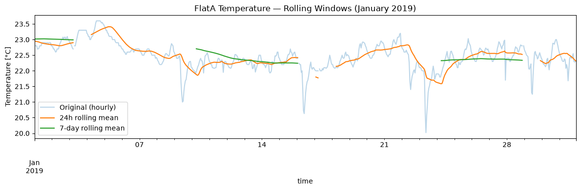
A rolling window computes a statistic (mean, std, etc.) over a sliding window of fixed size. This smooths noisy sensor data and reveals underlying trends — for example, a 24-hour rolling mean removes short-term fluctuations caused by window openings (visible as sudden temperature drops in the plot) and reveals the actual room temperature trend.
import matplotlib.pyplot as plt

# 24-hour moving average (1 day). window=24 counts rows: 24 rows are 24 hours here because
# every hour has a row (missing readings are NaN). For irregular data use rolling("24h").
df["FlatA_Temp_24h"] = df["FlatA_Temp"].rolling(window=24).mean()

# 168-hour moving average (7 days)
df["FlatA_Temp_7d"] = df["FlatA_Temp"].rolling(window=168).mean()

# Plot one month to see the effect clearly
df_jan = df.loc["2019-01"]

fig, ax = plt.subplots(figsize=(12, 4))
df_jan["FlatA_Temp"].plot(ax=ax, alpha=0.3, label="Original (hourly)")
df_jan["FlatA_Temp_24h"].plot(ax=ax, label="24h rolling mean")
df_jan["FlatA_Temp_7d"].plot(ax=ax, label="7-day rolling mean")
ax.set_ylabel("Temperature [°C]")
ax.set_title("FlatA Temperature — Rolling Windows (January 2019)")
ax.legend()
plt.tight_layout()
plt.show()

# Clean up helper columns
df = df.drop(columns=["FlatA_Temp_24h", "FlatA_Temp_7d"])
Handling Missing Data in Rolling Windows#
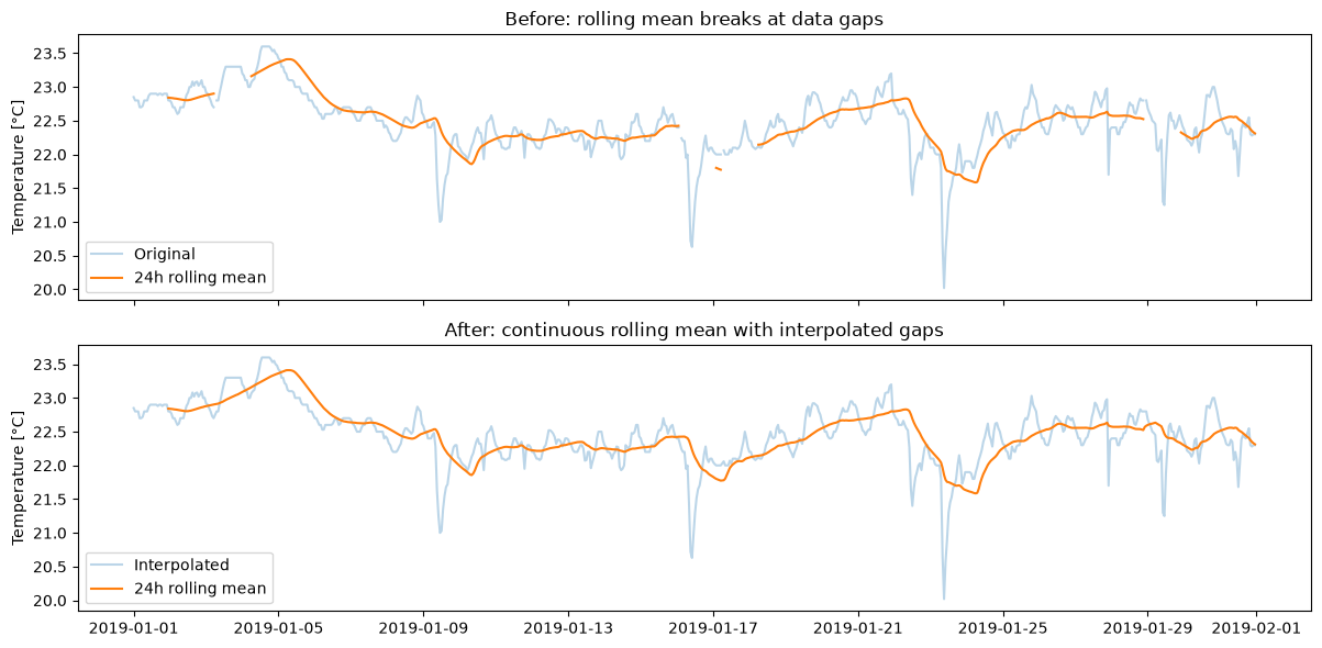
In the plot above, the rolling mean lines have gaps. This happens because .rolling() returns NaN whenever the window contains missing values — and real-world sensor data almost always has gaps (sensor offline, transmission errors, maintenance).
Before applying rolling windows, it is often useful to fill these gaps first.
# Check: how many missing values per column?
df_jan = df.loc["2019-01", ["FlatA_Temp"]].copy()

# Resample to explicit hourly grid to reveal hidden gaps
df_jan = df_jan.resample("h").mean()

print(f"Total rows:    {len(df_jan)}")
print(f"Missing (NaN): {df_jan['FlatA_Temp'].isna().sum()}")
print(f"Coverage:      {df_jan['FlatA_Temp'].notna().mean():.1%}")
Total rows:    744
Missing (NaN): 4
Coverage:      99.5%
# Fill gaps with linear interpolation
df_jan["FlatA_Temp_filled"] = df_jan["FlatA_Temp"].interpolate(method="linear")

print(f"Missing after fill: {df_jan['FlatA_Temp_filled'].isna().sum()}")
Missing after fill: 0
import matplotlib.pyplot as plt

# Compare: rolling mean with and without gap filling
df_jan["rolling_with_gaps"] = df_jan["FlatA_Temp"].rolling(window=24).mean()
df_jan["rolling_filled"] = df_jan["FlatA_Temp_filled"].rolling(window=24).mean()

fig, axes = plt.subplots(2, 1, figsize=(12, 6), sharex=True)

# Top: with gaps
axes[0].plot(df_jan.index, df_jan["FlatA_Temp"], alpha=0.3, label="Original")
axes[0].plot(df_jan.index, df_jan["rolling_with_gaps"], label="24h rolling mean")
axes[0].set_ylabel("Temperature [°C]")
axes[0].set_title("Before: rolling mean breaks at data gaps")
axes[0].legend()

# Bottom: filled
axes[1].plot(df_jan.index, df_jan["FlatA_Temp_filled"], alpha=0.3, label="Interpolated")
axes[1].plot(df_jan.index, df_jan["rolling_filled"], label="24h rolling mean")
axes[1].set_ylabel("Temperature [°C]")
axes[1].set_title("After: continuous rolling mean with interpolated gaps")
axes[1].legend()

plt.tight_layout()
plt.show()
Centered vs. Trailing Rolling Mean#
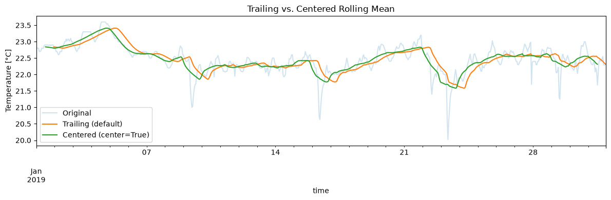
By default, .rolling() computes a trailing mean — it uses the current value and the N−1 values before it. This shifts the result to the right (it “lags” behind the data).
A centered rolling mean (center=True) uses values on both sides of each point, producing a symmetric smoothing without time shift.
# Trailing vs. centered rolling mean
df_jan["trailing_24h"] = df_jan["FlatA_Temp_filled"].rolling(window=24).mean()
df_jan["centered_24h"] = df_jan["FlatA_Temp_filled"].rolling(window=24, center=True).mean()

fig, ax = plt.subplots(figsize=(12, 4))
df_jan["FlatA_Temp_filled"].plot(ax=ax, alpha=0.2, label="Original")
df_jan["trailing_24h"].plot(ax=ax, label="Trailing (default)")
df_jan["centered_24h"].plot(ax=ax, label="Centered (center=True)")
ax.set_ylabel("Temperature [°C]")
ax.set_title("Trailing vs. Centered Rolling Mean")
ax.legend()
plt.tight_layout()
plt.show()
When to use which?
Method |
Code |
When to use |
|---|---|---|
Centered |
|
General smoothing and trend analysis — no time shift, shows the true trend at each point in time. Best for visualizations and reports. |
Trailing |
|
Causal analysis and real-time applications — only uses past data, which is physically meaningful. Use when modeling how outdoor temperature influences indoor temperature with a time lag (thermal inertia of the building). |
Example — building thermal inertia: A building does not react immediately to outdoor temperature changes. A trailing rolling mean of 24h outdoor temperature better represents the “effective” outdoor temperature that the building actually “feels” at a given moment. This lagged signal correlates better with indoor temperature or heating demand than the instantaneous outdoor temperature.
For pure data visualization and trend detection, centered is usually the better choice.
Gap filling strategies
Method |
Code |
Best for |
|---|---|---|
Linear interpolation |
|
Short gaps in smooth signals (temperature, humidity) |
Forward fill |
|
State data (on/off) — carries the last known state forward |
Spline |
|
More natural curves for sensor data |
Leave as NaN |
— |
Long gaps where interpolation would be misleading |
limit_area="inside" fills only gaps between two valid values; without it, pandas also
extends the last value over missing data at the end of a series.
Careful with limit: interpolate(limit=6) or ffill(limit=6) does not skip long
gaps: it fills the first 6 values of every gap, also of a two-day gap. To fill only gaps of
up to 6 hours and leave longer gaps as NaN, measure the length of each gap first:
s = df["FlatA_Temp"]
gap_len = s.isna().groupby(s.notna().cumsum()).transform("sum")   # length of each NaN run
filled = s.interpolate(limit_area="inside").where(s.notna() | (gap_len <= 6))